
IF YOU ARE HERE MAINLY FOR THE LOW-Z CALCULATOR REFERENCE, CLICK HERE.
Contents
Main Tab General Specifications
Introduction
Amplifier specifications can be difficult to decipher. They have evolved over decades, and many are so vague as to be useless for deploying an amplifier or comparing it with a competitive model. Since SynAudCon courses provide in-depth training on understanding amplifiers and how to select them, we started from the ground up when developing our training modules. By taking amplifier specifications back to the basics, you can understand what matters and what doesn’t with regarding to amplifier performance.
The Common Amplifier Format (CAF) is a report for presenting a set of specifications and measured performance metrics of audio power amplifiers. While some of this information can be found on manufacturer’s specification sheets, each manufacturer presents the information differently. In addition, the methods used to test the amplifier may be undocumented or vague, making it impossible to do meaningful comparisons between various makes and models. The CAF provides a structured, consistent and well-documented report of an amplifier’s performance.
The CAF is not a standard, but it can be used to report standardized specifications. Fields are provided to describe exactly what was measured and how.
Objective
The objective of the CAF is simple:
1. Provide the performance metrics needed to select and deploy an amplifier in a concise, well-defined and defensible format.
2. Provide performance metrics in a manner that facilitates apples vs. apples comparisons between makes and models.
There are many ways to measure amplifiers and specify their performance. Many amplifier manufacturers have excellent specification sheets available to the system designer. Even if the CAF simply replicated this information, it adds depth and formalizes the presentation, freeing the user from having to decipher these often cryptic spec sheets.
No set of specifications can replace the listening process for evaluating an amplifier or comparing amplifiers. If you want to know how two amplifiers compare in reproducing an intense kick drum signal into a 2 ohm subwoofer, you should hook them up and conduct proper A/B listening tests. The CAF can serve as a front end for this exercise, or as a back end. It bridges the gap between artistic evaluation and technical deployment. Both are vital to the sound system design process.
CAF Philosophy
Amplifiers Drive Loudspeakers
An amplifier can be designed and measured as though it will only drive a simple resistive load. In actual use it must drive a complex, reactive, electro-acoustic system. This affects one’s philosophy with regard to amplifier loading. It’s not just about “getting the most watts.” The prime directive is achieving fidelity when converting the electrical signal into an acoustic one. This means preserving the voltage characteristic of the waveform by making the amplifier immune to the loudspeaker’s impedance curve. When it comes to power amps, there are important differences between heating resistors and driving loudspeakers. With the former, the objective is power transfer. With the latter, the objective is waveform preservation, or in other word’s – voltage linearity.
Power Ratings
The term “power” amplifier is a bit of a misnomer. It’s not amplifying power. In reality it is producing a higher voltage facsimile of the input voltage waveform, with sufficient current to meet the demands of the load impedance. The amplifier/loudspeaker interface is optimized for voltage transfer, and all of the measurements included in the CAF are made with a voltmeter, albeit a very capable one.
The amplifier’s output voltage can be tested open circuit (no load) or into any load resistance. The manufacturer determines the supported load resistances. If the resistance gets too low, the amplifier may current limit and its voltage may drop, making it non-linear in response. A 5-part video series that describes this in more detail can be found here.
The importance of understanding the principles of a voltage transfer interface cannot be over-stated. All audio signal processes are voltage modifiers. This includes graphic equalizers, parametric equalizers, and IIR and FIR digital filters. Voltage changes made by these devices translate directly to the frequency response of the loudspeaker, and (should be) independent of the loudspeaker’s impedance curve. As such, as goes the voltage, so goes the signal produced by the loudspeaker. SPL calculations should always be performed using the RMS voltage of the signal from the amplifier. The voltage power matrix of the CAF is built upon this principle.
The CAF requires the use of three signal types for testing the amplifier. A burst test reveals the voltage amplitude capabilities of the amplifier without requiring that it source much current over time. A continuous sine test reveals the current production capabilities of the amplifier under load. It’s a torture test! The pink noise test reveals the performance of the amplifier at approximately 1/8 power, which is typical for slightly clipped or compressed music or speech program material. Without all three tests, amplifiers that are quite different can look very similar.
Distortion Specifications
A distortion measurement basically describes the difference between an amplifier’s input and output signal. If they are the same, other than the voltage gain, then there is no distortion. There are several distortion types, including Total Harmonic Distortion (THD) and Intermodulation Distortion (IMD). Volumes have been written on both. There exists no universally accepted criteria for the amount of distortion that can be tolerated, but all agree that it should be very low.
It’s easy to get bogged down with regard to the amount of “allowable” distortion. Modern amplifiers can have very low distortion ratings. For the purpose of establishing rated power, an excellent distortion analyzer is an oscilloscope. Distortion becomes obvious when the waveform is a sine wave. Visual deformation tends to correlate with 1% THD. The nature of THD is that it drops VERY rapidly as the signal is reduced, so if the amplifier is turned down only 0.1 dB the THD probably drops significantly. Rather than get mired in distortion specsmanship, the CAF ratings are based on 1% THD. If this is not attainable then the actual distortion is indicated in the provide notes fields.
So, the CAF philosophy is that 1% THD is low enough for measuring the amplifier’s output voltage for the purpose of establishing the amplifier’s rated power, which is in turn de-rated by the crest factor of the program material for SPL calculations. The manufacturer’s data sheet can be consulted in cases where more information on the distortion performance is desired.
There’s no need to use a microscope when a magnifying glass will do.
CAF Conventions
The Expression of Audio Levels
There are several choices for specifying the voltage and power levels produced by audio products. Voltage is commonly expressed in dBV or dBu. Power is expressed in dBW or dBm. All voltages in the CAF are root-mean-square unless otherwise indicated (Vrms).
There is no universal agreement on which of these should be used to present the amplifier’s specifications. That’s why CAFViewer allows the user to decide, providing radio buttons to choose between Vrms, dBV, and dBu.
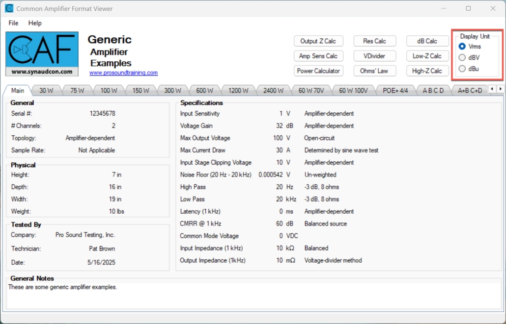
Figure 1 – Voltages can be displayed as Vrms, dBV, or dBu.
CAFViewer™ Layout
The CAF is divided into three major sections, organized by tabs. The number of tabs grows dynamically depending on the amplifier, but more about that later.
1. The Main Tab
2. The Frequency Response Tab (optional)
3. The Voltage, Power I/O Matrix Tabs
Here is an overview of each.
The Main Tab
This “home” page of CAFViewer gives information on the general characteristics of the amplifier, including some “one number” performance metrics. Please refer to this graphic for a description of each.
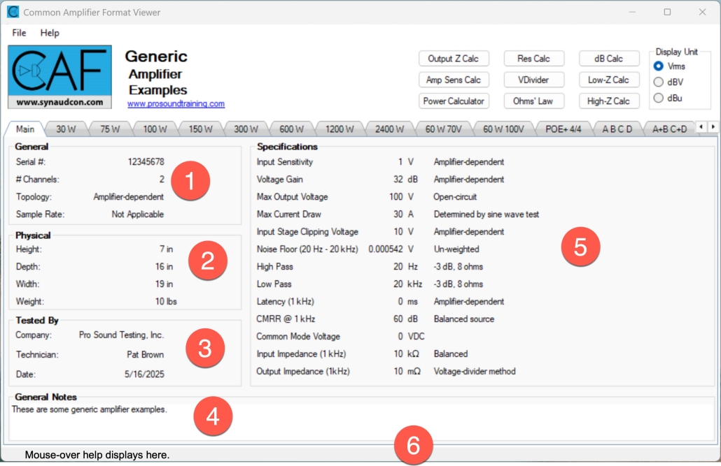
Figure 1 – Overview of CAFViewer™ main page.
1 – General
These are general characteristics of the amplifier as provided by the manufacturer, including the serial number of the unit tested. The amplifier topology is given, along with the sample rate (for digital devices).
2 – Physical
These are physical characteristics of the amplifier as provided by the manufacturer.
3 – Tested By
This is the party that performed the testing, along with the date.
4 – General Notes
Additional information that does not conform to the other sections can be included here.
5 – Specifications
These are “one number” metrics used to summarize a characteristic of the amplifier. Each is explained in a section below.
6 – Mouse-over Help
This section shows information about the various ratings, plots, etc. throughout the entire calculator.
The Frequency Response Tab
The Frequency Response tab is optional and may not be included with an amplifier CAF file. It can be used in various ways depending on what the manufacturer is trying to convey. It is free form by design, and can be used to plot any voltage vs. frequency.
All amplifiers are 20 Hz – 20 kHz, right? Not so! Amplifiers designed to drive transformer distribution systems often have an intentional low frequency roll off. Subwoofer amplifiers are band-limited, and often include an equalization curve. An amplifier’s frequency response may change with drive level. To remove any doubts the Frequency Response Tab can display the transfer function of the amplifier under many stated conditions.
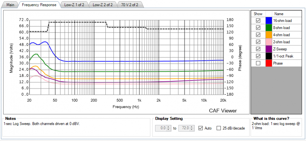
Figure 3a – Overview of CAFViewer™ Frequency Response Tab
The following show some possible uses of the Frequency Response tab.
1 – Up to 6 Plots
This plot is produced by feeding the amplifier a log sweep at its full input sensitivity. Note that the Y axis can be scaled in Vrms, dBV, or dBu. The load resistance and THD for the full voltage sweep is listed in the Notes section. While this is a free-form tab, it is revealing to produce a plot with the amplifier loaded at Zmin, 2Zmin, and 4Zmin. This reveals its ability to maintain its output voltage under load.
2 – Z-Sweep Response
Another interesting plot is with the amplifier loaded by a reactive load at its Zmin. In Figure 3a the purple curve shows the amplifier’s voltage tracking the impedance curve where as ideally it should be independent of the impedance curve.
3 – Peak Output Voltage
This plot displays the results of Don Keele’s Peak Tone Burst test. It displays the measured peak output voltage of the amplifier on 1/1-octave centers. These are the only peak voltages in the CAF, and they are measured, not calculated.
4- Phase Response
A complete transfer function contains both magnitude and phase information. The phase response plot is produced from the same sweep as the Full Voltage response. For critical applications the phase response at the frequency extremes may need to be considered, since high pass and low pass filters are required to band limit the amplifier. Please note that it can be toggled off if desired.
5 – 25 dB/decade Plot Aspect Ratio
Selecting this displays the frequency response using the IEC 60268-5 Standard. This prevents “over-smoothing” of the frequency response by using an excessive range on the Y-axis, which can make an amplifier or loudspeaker appear “flatter” than it actually is.
From Don Keele, Jr.:
EC 60263 (graph aspect ratio) is a normative reference in IEC 60268-5 (loudspeakers), and has been for over 30 years. It’s actually normative throughout all of the 60268 series in IEC TC-100 as well as all of the standards in IEC TC-29 (hearing aids, measurement microphones, etc.).
It is also a normative reference in the new IEC 60268-21 and draft IEC 60268-22 revisions/updates of IEC 60268-5 that our working group chaired by Wolfgang Klippel is working on. (Of course, that alone is no assurance that anyone will actually follow it…).
This is an information dissemination / education problem: The vast majority of technical people working in this area are completely unaware of the IEC 60263 standard, which has been around a very long time and dates to the period of level recorders where the size of the recording paper fixed the aspect ratio, and not surprisingly, came in 3 sizes, corresponding to the 10, 25, and 50 dB per decade aspect ratios. You can see this ‘violation’ in many JAES papers as well. One has to force this manually in MS Excel, the latest versions of which also have a bug in the log x axis routine (selecting 20 Hz as the starting frequency puts all of the grid lines in multiples of 2 even if a base of 10 is selected…). It’s a wide-spread problem.
The “Z-Sweep”
The CAF now supports a test that I call “Z-sweep.” While amplifier testing is historically performed into resistive loads (for good reasons) the Z-Sweep test uses a reactive load. The Z-Sweep measures the amplifier’s frequency response into a real-world reactive load – one whose magnitude and phase responses change dramatically with frequency. This type of load should have no significant effect on the amplifier’s frequency response. In other words, an amplifier’s frequency response should be independent of the shape of the impedance curve. If this is not the case, then the amplifier would have a different frequency response into various “4-ohm” loudspeakers, each of which has a unique impedance curve.
Another reason for the Z-Sweep test is that the rated impedance of a loudspeaker is about 20% higher than its minimum impedance (Zmin). A “4-ohm” loudspeaker can have a Zmin of 3.2 ohms. The Z-Sweep impedance is calibrated to Zmin, representing a worst case for the amplifier to drive. It reminds us that amplifiers are designed to drive 4-ohms so that they can drive real-world 8-ohm loads whose impedance can dip down to 6.4 ohms. Two real-world 8-ohm loads in parallel (3.2 ohms) will overload most amplifiers for some types of program material.
Figure 3b shows the transfer function of the reactive dummy load impedance. Figure 3c shows the amplifier’s response into a resistor compared to the reactive load. The sweep duration is 1 second. Differences of less than 1 dB can be ignored.
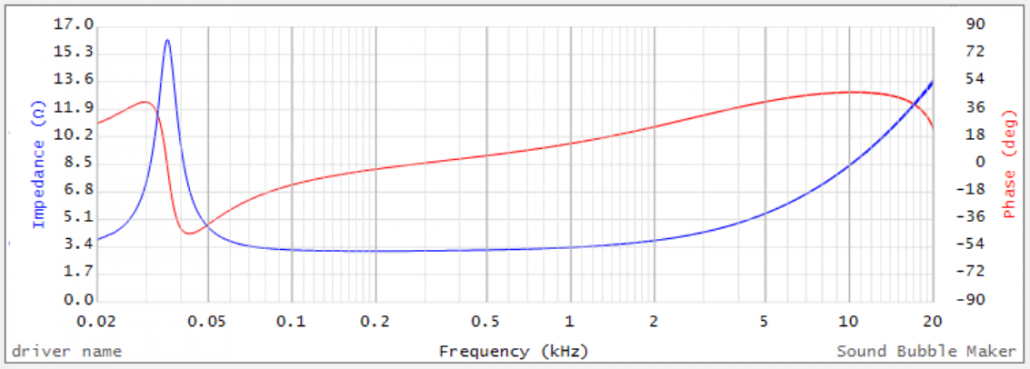
Fig. 3b – The impedance magnitude and phase of the Z-Sweep reactive load, calibrated to 4-ohms.
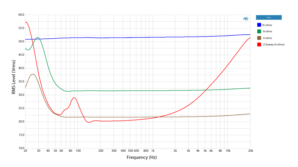
Fig. 3c – A comparison of the response of an amplifier into various load resistances, including the Z-sweep load. The drive signal is a 1-sec log sweep. An idealized “perfect” amplifier (doesn’t exist) will produce the same response for all four loads.
The I/O Matrix Tabs
The heart of the CAF is the voltage/power input output matrix. Each operating mode of the amplifier gets a tab. Modes are defined by whether or not a hardware or software switch is selected to change the amplifier’s behavior. In short, if you have to throw a switch it’s now a different amplifier, and it gets its own tab. The number of tabs grows dynamically depending on the amplifier, and some amps have many!
It is also possible to display more than one amplifier in the same CAF file. The default “Generic Amplifier Examples” file that loads with the CAFViewer is an example. A manufacturer may choose to publish one file that contains a whole series or even their entire product line. It’s up to them.
There are two amplifier types used in audio. If the tab says “Low-Z” then the amplifier connects directly to a loudspeaker with a low impedance value, such as 8 ohms. If the tab says “High-Z” then the amplifier connects to a loudspeaker(s) through a step-down transformer. This transformer is usually packaged with the loudspeaker.

Figure 4 – The I/O matrix tabs. By default CAFViewer opens with tabs for common amplifier types and sizes.
We’re now ready to have a look at the first section of the I/O matrix. This example uses a Low-Z tab, and you can see the supported resistances in column 3. These are determined by the manufacturer. If they claim 2-ohm support, they must provide some measured data!
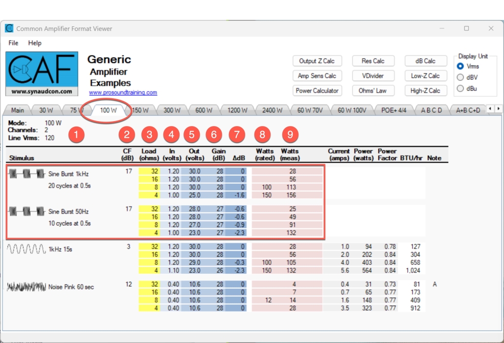
Figure 5 – Burst section of I/O matrix.
Burst Test Results
1 – Stimulus Type – The CAF requires that the amplifier be tested with 3 stimulus types. First on the list is a burst test. There is flexibility on the details of the burst, but CTA-2006-D serves as a good guideline. A 1 kHz 20 cycle full-scale burst is interleaved with 480 cycles at -20 dB.
2 – Crest Factor – This is the peak-to-RMS ratio of the stimulus. The higher the crest factor, the lower the signal RMS voltage and power.
3 – Load Resistance – This is a resistive load, with an adequate power rating and cooling to handle the amplifier’s output signal. The manufacturer determines the lowest resistance for testing the amplifier.
4 – Input Voltage – The voltage applied to the amplifier input to produce its output voltage. The input voltage can be reduced as needed to stay below 1% THD.
5 – Output Voltage – The RMS voltage of the full-scale burst segment is analyzed to determine the amplifier’s RMS output voltage.
6 – Gain – This is the ratio of the output voltage to the input voltage, expressed in relative dB.
7 – Loading Effect – The amplifier shown is first tested with a 32 ohm load (4x its maximum load of 4 ohms). This relatively light load allows the amplifier’s full output voltage to be determined without stressing the amplifier. The load is then halved (16 ohms) and the test repeated. The process is repeated until the maximum load (minimum Z) is reached.
By default the first line of the matrix (32 ohm load) is the reference (0 dB) and the voltage measured using the lower impedance loads are compared to it. If the Loading Effect value goes negative, it means that the output voltage dropped (due to the increased current demand).
The user may double-click any value in the Loading Effect column (burst or sine tests) to make it the reference value. The remaining values are now re-scaled relative to the chosen reference. This can allow a sine wave rating to be used as the reference, with the burst rating indicating “dynamic headroom.”
8 – Rated Power – This is the power rating given the amplifier by the manufacturer. Columns for which there is no rated power are blank. Most amplifiers have an 8 ohm rating. Many are rated at 4 ohms, and some are rated at 2 ohms. The 8 ohm rating is of interest when working with EASE GLL™ files.
9 – Measured Power – This is the power calculated by squaring column 5 and dividing by column 3. Ideally the measured power should equal or exceed the rated power. It should be noted that for a burst test this “power” rating is only for a short waveform segment, which due to its short duration doesn’t generate much power. It is a reference value that should be de-rated by the crest factor of the program material (6 – 20 dB). For the true output power, please see the segment on “Continuous Sine Results” below.
Continuous Sine Results
The next section of the I/O matrix reveals the results of the continuous sine test. At one time virtually all amplifier testing was done with continuous sine waves. With a 3 dB crest factor, it is the electrical equivalent of a mechanical drop test, essentially torturing the amplifier. There exists no universal agreement on the length of the test, but the CAF recommends at least 15 seconds. The time span and %THD are indicated in the appropriate fields.
Here is an excellent blog on “Why Sine Waves?”
The test requires that the amplifier maintain the same amplitude over the time span. If the voltage drops during the test, the test is aborted and after an appropriate wait it is repeated with a 1 dB lower level drive signal. This is why the matrix includes both the input and output voltage. The input voltage that produces the sustainable output voltage becomes the amplifier sensitivity for that particular test. Ideally, the continuous sine test results should be very similar to the sine burst results.
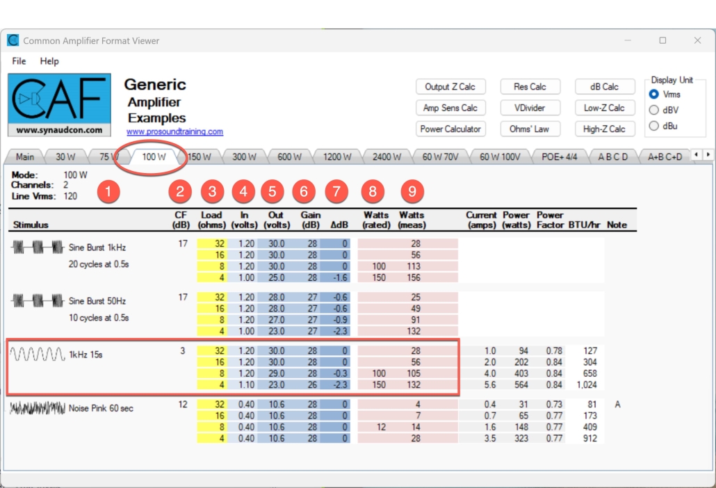
Figure 6 – Continuous Sine test results.
Utility Power
Amplifier’s don’t “make” power. The draw power from the utility power circuit and convert it into audio power. The CAF measures the power draw for the continuous sine wave and pink noise signals. Some additional columns are added to the continuous sine matrix (Fig. 7). They are described below.
10 – Amps – This is the current drawn from the utility power circuit during the test. It provides a guideline for the selection of the circuit breaker for the amplifier, representing a worst-case scenario with regard to power draw.
11 – Watts – This is the power drawn from the utility power circuit during the test. Note that audio power (column 8) will always be less than column 11, unless you’ve figured out a way to get the amplifier to create power. If so let’s talk. I’ll invest.
12 – Power Factor – A DC source has a power factor of 1. AC sources have a power factor of less than 1. If the amplifier incorporates power factor correction, it will show up here.
13 – BTU/hr – This is the heat output of the amplifier, useful for designing a cooling system. The sine wave stimulus represents the worst case scenario. It can be de-rated as desired. See the next section on Pink Noise stimulus. For our international friends, BTU/hr can be converted to kCal/hr by multiplying by 0.25. I originally included it but needed to save space.
14 – Any special notes regarding test conditions, nuances, special setups, etc. can be listed below the matrix.
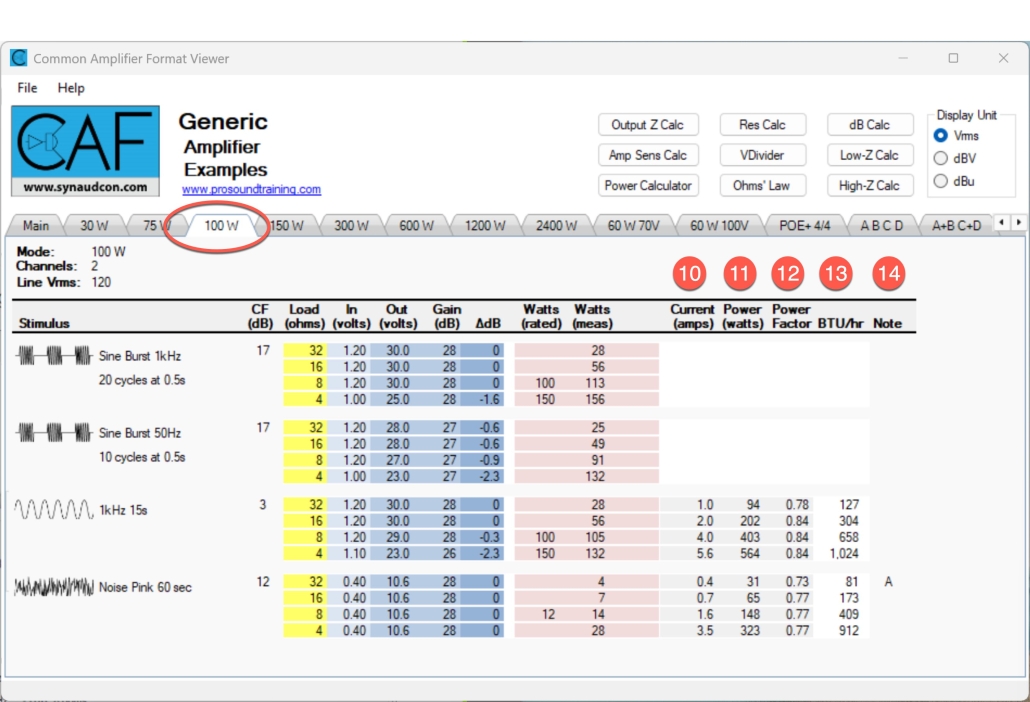
Figure 7 – Additional columns are provided to characterize the utility power consumed by the amplifier.
A Note Regarding Sine vs. Burst Test Results
The matrix reveals that the burst power is often higher than the continuous sine power. In reality the opposite is true, since the burst output considers only 20 ms (1 kHz). A system cannot output more power than it draws. The burst test presents the signal power as though the burst segment were continuous. For sine wave power, it actually is continuous. For an idealized amplifier, the voltage (and resultant power) will be the same.
Pink Noise Results
The pink noise results usually best represent how most amplifiers are actually used. Pink noise simulates program material with a 12-14 dB crest factor. This “noise power” is typically 1/8 rated power.
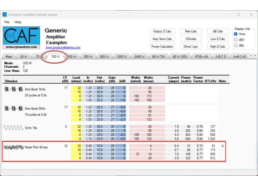
Figure 8 – Continuous Pink Noise Test Results
The signal is broad band, and the crest factor is 6-12 dB. This produces about 1/8 the audio power of a sine wave. To better simulate music and speech program, the noise may be shaped (e.g. IEC-268-1 noise) and the crest factor limited to 6 dB (50332 noise). This can prevent the activation of limiter circuits within the amplifier which can prevent the amplifier from reaching “1/8 power.” When reproducing noise, the amplifier is operating far below its full power output – just coasting when compared to a sine wave. The CAF allows any noise type and duration to be used, so long as it is specified in the matrix.
As you can see, the current draw for noise is much lower than that of a sine wave. This represents a good lower limit for sizing circuit breakers and cooling systems.
Idle
The power draw and BTU output for the amplifier at idle may also be included in the matrix. Note that the voltage field will usually indicate “0 Vrms” but if you select dBu or dBV you will see a very low level, an excellent example of why we prefer to work in dB. Additional lines may be included if the amplifier has a “green” mode, etc.
The idle section is optional and its inclusion is left to the discretion of the manufacturer.
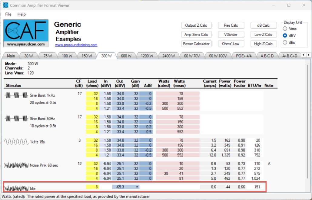
Figure 9 – Amplifier output at idle. The rows in the matrix can grow indefinitely. Additional sections can be added for any stimulus type.
Multiple Tests Tell the Story
The CAF report reveals a lot about an amplifier’s performance. The output voltage is measured under multiple conditions with multiple waveforms and the system designer is free to consider any or all of them.
Burst Test – short term output voltage into indicated load. This is useful for finding the amplifier’s maximum output voltage without stressing it.
Sine Test – continuous output voltage into indicated load and for indicated duration. This is useful for finding the amplifier’s maximum output current. It is a stress test when into lower load impedances.
Noise Test – output voltage for noise stimulus. This is most like the day-to-day use of most amplifiers.
High-Z Amplifiers
If the tab says “High-Z” “70V” or “100V” then the amplifier is designed to drive loudspeakers that incorporate step-down transformers.
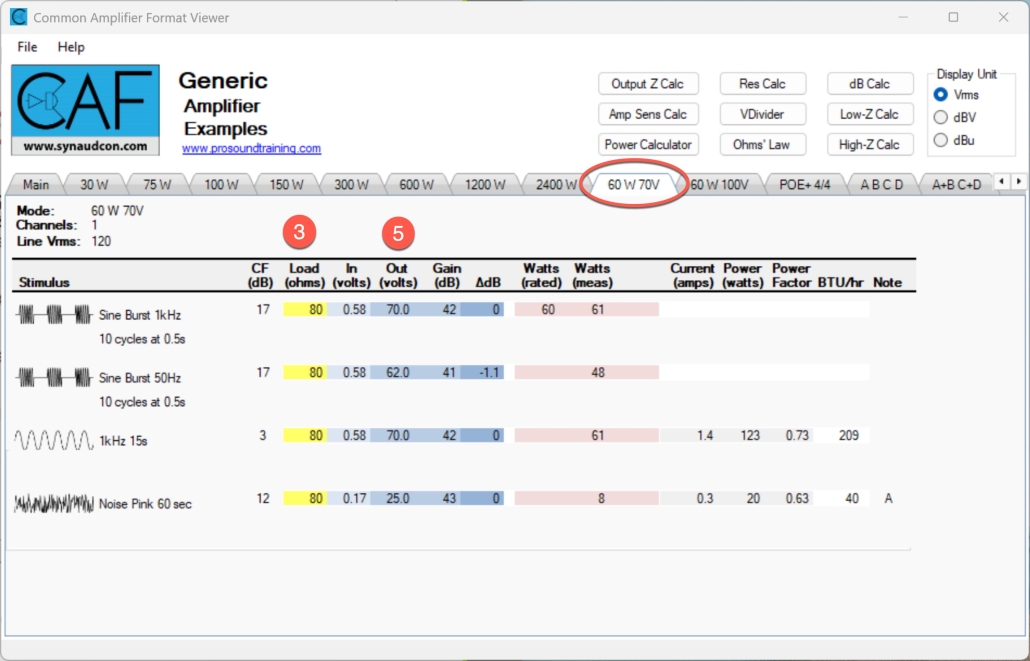
Figure 10 – The tab for a High-Z amplifier.
A High-Z tab is essentially the same as a Low-Z tab with regard to most measures, but you will notice the output voltage is a standard value used in distribution systems, such as 70 V or 100 V. You will also notice that the Load R (column 3) is typically higher than for Low-Z amplifiers (hence the name). In principle High-Z distribution works the same as Low-Z distribution, except the circuit values (voltage and impedance) are scaled to higher values. This provides several benefits and one drawback.
Benefit – The higher load impedance permits the use of smaller diameter cable.
Benefit – Multiple loudspeakers can be daisy-chained onto a single amplifier, with the volume of each selected at the loudspeaker by a “power tap” such as 1 W, 2 W, 4 W, etc.
Drawback – The reactive properties of the step-down transformer may limit the low frequency response when compared to a Low-Z interface.
In principle, as “small” wattage amplifier can have a high output voltage, but the load impedance must be high enough to prevent the amplifier from current-limiting.
These systems are typically designed by making sure that the sum of the loudspeaker power taps placed on the line does not exceed the amplifier’s rated power. Easy enough. This is exactly how electricians determine the load on a household utility power circuit. For this reason, many high-Z amplifiers only give the distribution voltage and rated power. The CAF takes it a step further, showing the minimum load impedance (as determined by the power rating) that the amplifier can drive at its distribution voltage (column 15). This benefits the designer that must deploy an amplifier into an existing system where the number and location of loudspeakers is not known. An impedance measurement of the line reveals the load that the amplifier must be able to drive, and summing the power taps is unnecessary (and maybe impossible).
For a fuller description of High-Z distribution, see the section on the High-Z calculator.
The CAF Calculators
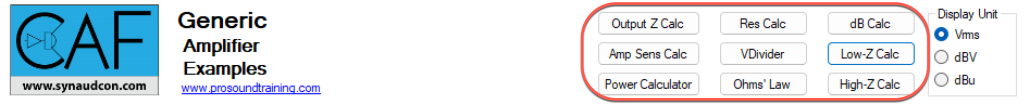
CAFViewer includes calculators for both low-Z and high-Z distribution systems. Their operation is described below.
The Low-Z Calculator
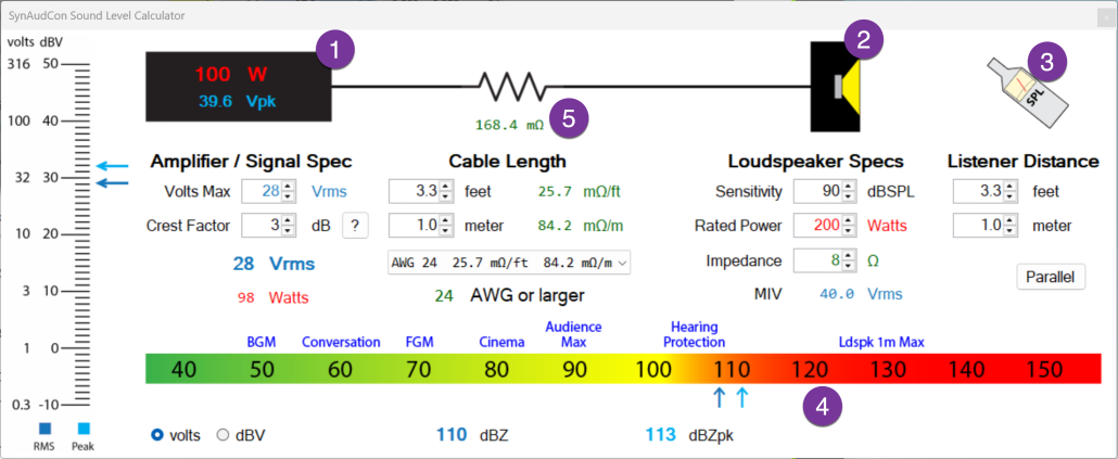
Figure 11 – The Low-Z Calculator
Section 1: Amplifier – The fields and graphics below and to the left of the amplifier graphic are variables related to the amplifier. The field for “sizing” the amplifier is “Volts Max.” The amplifier signal is specified in RMS volts. This is the maximum sine wave (or burst) voltage from the amplifier. On the amplifier graphic (the black box) the 8 ohm power rating for this voltage is indicated in red and the peak voltage of the sine wave is indicated in blue.This establishes an extremely useful relationship between voltage (sine wave) and power (8 ohm).
So, you “size” the amplifier by changing the voltage. Increase (or decrease) the Volts Max until the desired power is reached (red text on amplifier). This may seem strange at first, but it promotes correct thinking about how amplifiers work. To work with a particular amplifier, find the 8 ohm power rating from the manufacturer’s data sheet and scale the Volts Max until you reach that wattage. The Volts Max will equal the amplifier’s maximum sine wave voltage. You can now work in volts RMS instead of watts.
Both the peak and RMS sine wave voltages are displayed on the voltmeter to the left of the graphic. By sizing the amplifier using the Volts Max, you are establishing the rated condition for the amplifier or a sine wave (or sine wave burst). You can now increase the CF to simulate real-world program material.
The CF is the peak-to-RMS ratio of the audio signal. The crest factor (CF) selector reduces the RMS voltage as you increase it. You can watch it happen on the voltmeter. Increasing the CF is what gets us from a rated condition for the amplifier (sine wave), to an actual use condition (speech or music). A table of typical crest factors pops up when you click on the “?” button.
The new (reduced) RMS voltage is displayed below the CF selector in blue. It is also presented as a wattage into 8 ohms (red). This RMS voltage determines the sound pressure level (and heat) produced by the loudspeaker.
The crest factor defaults to 3 dB (sine wave). It should be increased to describe the program material you intend to feed the amplifier. Here are some examples.
0 dB – Square Wave (for theoretical purposes only!)
3 dB – Sine Wave (the reference condition for the amplifier)
6 dB – 1/2 Sine Power (HEAVILY compressed program material)
9 dB – 1/4 Sine Power
12 dB – 1/8 Sine Power (moderately compressed or clipped program)
15 dB – Slightly compressed or clipped program
>18 dB – Uncompressed music or speech.
Note the volts/dBV meter next to the amplifier graphic. This displays the amplifier’s signal as a voltage, as used by EASE GLL, the Common Loudspeaker Format, and AES 75. These resources use voltage ratings in lieu of power ratings for sizing amplifiers and loudspeakers. The volts/dBV radio button switches between volts and dBV.
Section 2: Loudspeaker – The fields below the loudspeaker graphic are the loudspeaker variables. This is where the rated 1 m sensitivity is entered. It should be provided by the manufacturer or can be read from the GLL or CLF data file. This is normally the average sensitivity – a one number rating for a flat line drawn through the sensitivity plot. The sensitivity is measured by applying a 2.83 sine wave (tone) to the loudspeaker at a specified frequency resolution. Figure 12 shows the 1/3-octave sensitivity for a sound reinforcement loudspeaker.
The rated power handling is entered below the sensitivity field (red). This can be found on the loudspeaker’s specification sheet. The loudspeaker impedance field defaults to 8 ohms, and it should normally be left there, no matter the rated impedance of the loudspeaker. The exception is when you are calculating the needed wire gauge in section 5. For this, enter the loudspeaker’s lowest impedance over its rated bandwidth. The Maximum Input Voltage (MIV) is calculated from the rated power and displayed in blue. This is the maximum RMS signal voltage that the loudspeaker can safely handle. It is determined by the thermal limits of the loudspeaker. This is the value used in an EASE GLL file for calculating the maximum RMS SPL from the source.
If you know the MIV, you can simply increase the rated watts variable until you reach it. This makes the Rated Power and MIV alternative ways of looking at the same thing – a VERY important point.
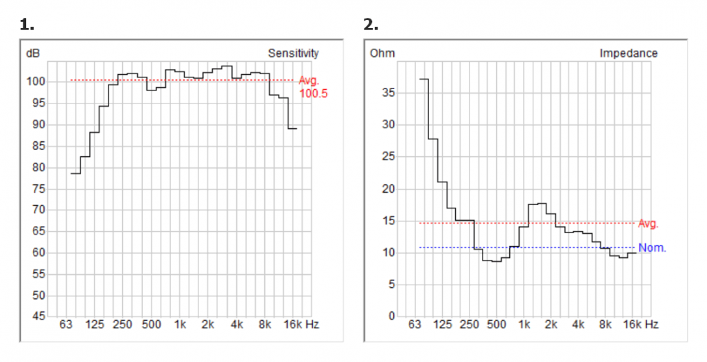
Figure 12 – Rated sensitivity and impedance taken from CLF Viewer. This loudspeaker would be treated as “8 ohms” for sensitivity and MIV specifications.
Section 3: Listener Distance – Note that the Listener Distance defaults to one meter. This is the reference distance for the loudspeaker sensitivity. The listener distance is increased in either feet or meters. The calculator assumes inverse-square law level change with distance (-6 dB per double distance). This is the behavior of a “point source” – a device that emits spherical sound waves when observed from the loudspeaker’s far field.
Section 4: Calculated SPL – The SPL is calculated and indicated on this scale. The RMS SPL is the primary result. It is given in dBZ (an RMS un-weighted level). The peak SPL is also given because it gets a lot of press. The actual maximum peak voltage has several dependencies, so don’t read too much into it. The approximate mid frequency levels for various program types are shown above the scale.
Section 5: Wire Gauge – The required wire gauge (American Wire Gauge AWG) based on the cable length and loudspeaker impedance is given here. Enter the appropriate impedance in Section 2. The CAF follows the 5% rule, where the allowable wire resistance should not exceed 5% of the loudspeaker’s impedance. This represents a line loss 0.5 dB. Watch the required AWG increase (lower number) as you increase the Cable Length.
The High-Z Calculator
The High-Z calculator is a modified version of the Low-Z calculator. The are two important differences (Figure 13).
- The amplifier voltage defaults to a standard distribution voltage (e.g., 25 V, 70 V, 100 V, etc.).
- The signal chain includes a step-down transformer.
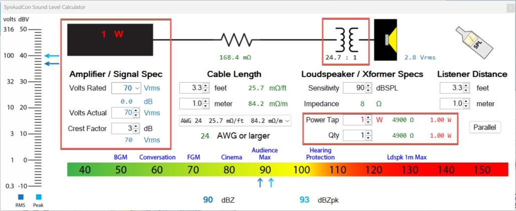
Figure 13 – The High-Z calculator
All other calculations are the same as the Low-Z calculator. There’s an important lesson in that fact. Low-Z and High-Z distribution systems are very similar in operation. The difference is that a High-Z system starts with a rated distribution voltage, which is scaled to a lower voltage by the step-down transformer.
Loudspeakers for these systems typically have user-selectable “power taps” on the loudspeaker itself. The values imprinted on the loudspeaker are based on an assumed distribution voltage (e.g., 70 Vrms) and crest factor (3 dB) and the action of the step-down transformer. The High-Z calculator displays the turns ratio of the transformer, based on the power tap entry. While one doesn’t necessarily need to know the turns ratio, we include it for academic reasons.
Note that the transformer dramatically increases the impedance of the loudspeaker as seen by the amplifier, while at the same time stepping down the amplifier voltage delivered to the loudspeaker. It’s a two-way street. Since the loudspeaker now has a higher impedance, multiples can be paralleled onto a single amplifier. The Qty field allows you to select the number of loudspeakers. The total impedance of the line is shown, along with the total of the power taps, which is displayed under the amplifier graphic. Make sure your amplifier can source more power than what is drawn by the zone of loudspeakers.
Note that with the higher impedance values, a small wire gauge can often be used. CAFViewer calculates the wire gauge based on the total impedance of the zone.
An Important Note Regarding SPL
Even though a High-Z system is based on a standard reference voltage, you can still vary the SPL (down direction only!) with the amplifier’s volume control. The SPL will also be affected by the crest factor of the program material. In effect, it’s a sine wave rated system that may never see a sine wave, with the net benefit being the ability to drive multiple loudspeakers through a smaller diameter wire. Pretty cool, but these systems sometimes do not fare well for low frequency reproduction (<80 Hz) so check your component specs if that is important.
Main Tab General Specifications
1.1 – Input Sensitivity
This is the input voltage required to drive the amplifier to its full output voltage, into the indicated load impedance (typically 8 ohms). It is provided by the manufacturer, and verified by measurement. The input attenuator is typically at its maximum setting.
1.2 – Voltage Gain
This is the gain of the amplifier, found by
G = 20log(Eout/Ein)
Where:
G is the voltage gain of the amplifier in dB
Eout is the output voltage of the amplifier
Ein is the input voltage to the amplifier
Voltage gain is dependent on the setting of the input sensitivity control. Voltage gain tends to be independent of the drive level to the amplifier. The voltage gain is useful when signal processors such as compressor/limiters are placed ahead of the amplifier. The amplifier can then be treated as a simple “voltage gain block” and the output voltage of the amplifier determined by the signal processor block. This can be used to protect loudspeakers from excessive peak levels, RMS levels, or both.
Note: Many amplifiers have a user-selectable input sensitivity range. The manufacturer specifies which setting is used for the CAF testing.
1.3 – Max Output Voltage
This is the maximum linear sine wave output Vrms of the amplifier at 1 kHz with no load or the indicated load. It’s what the amplifier would output if it were used to drive an electronic input such as another amplifier (through an appropriate attenuator if necessary). The “no load” output voltage of the amplifier is useful for comparing to a “under load” condition. The voltages should be the same or similar.
1.4 – Max Current Draw
The maximum current draw from the AC power circuit as specified by the manufacturer, or as measured during the “all channels” sine wave test. The comment field provides the details
1.5 – Input Stage Clipping Voltage
This is the input voltage to the DUT at which the input stage of the amplifier clips. It is required because it may be possible to clip the amplifier’s input stage, prior to clipping the amplifier’s output stage. For example, if a mixer is producing +28 dBu, but the amplifier input stage clips at +12 dBu, the signal will be distorted no matter the setting of the amplifier’s gain control.
For this test the input sensitivity of the DUT is set at -20 dB ref. full output to prevent the output stage from clipping. A low level 1 kHz signal is applied to the DUT and slowly increased. The output voltage is monitored on an oscilloscope for visible clipping, which terminates the test. The input voltage is then measured and recorded.
1.6 – Noise Floor
This is the residual or “self-noise” of the amplifier. All electronic devices produce output noise, even without the presence of an input signal. For this test, the amplifier’s input is terminated by a low value resistance (e.g. 150 ohms) and the output voltage measured using a sensitive voltmeter. The input sensitivity should be set at maximum. If a weighting scale is used, it should be indicated in the notes field.
1.7 – High Pass
This is the -3 dB point on the high pass portion of frequency response curve. For many amplifiers it will be below the 20 Hz – 20 kHz bandwidth shown on the Frequency Response tab.
1.8– Low Pass
This is the -3 dB point on the low pass portion of frequency response curve. For many amplifiers it will be below the 20 Hz – 20 kHz bandwidth shown on the Frequency Response tab.
The amplifier’s overall bandwidth can be determined by subtracting the high pass frequency from the low pass frequency.
1.9 – Latency
Latency is the inherent, unavoidable delay of a signal passing through a digital amplifier. It is found by measuring the amplifier’s impulse response (IR). The IR can be presented in the frequency domain as group delay.
Note: The GD plot should be flat at the frequency at which the “one number” latency is determined. Since the GD is often frequency-dependent due to the high pass response of the amplifier, a frequency other than 1 kHz may be used, and should be indicated.
1.10 – Common-Mode Rejection Ratio (CMRR)
For a balanced input, the output level of a common-mode input signal relative to a differential-mode input signal. This is a “one number” metric for 1 kHz. While there are several methods for measuring CMRR, the IEC 60268-3 method is recommended. This places a 10 ohm imbalance in the output driving the amplifier.
1.11 – Common Mode DC Voltage
Some amplifiers have a common mode DC voltage on their loudspeaker output terminals. The loudspeaker doesn’t see it because it is connected in differential mode. For such amplifiers it is IMPORTANT to not ground either output terminal.
1.12 – Input Impedance (Zin)
The load impedance (electrical) presented to a source (e.g. mixer, DSP) by the input stage of the amplifier. It is of interest when the system design calls for multiple amplifier inputs to be driven from a single output. Typical values are 5kΩ and higher.
1.13 – Output Impedance
The output impedance of the amplifier is the source impedance seen by the load (such as a loudspeaker), neglecting the resistance of the interconnecting cable. Why is this here? In the case of power amplifiers it is typically extremely low and has no real effect on the voltage delivered to the load. It is more traditional to specify a “damping factor” for an amplifier, which is the ratio of the load resistance to the amplifier’s output impedance, with a higher number being “better.” But, this is an abused specification that is no longer taken seriously by most engineers, since the amplifier’s output impedance is swamped out by other resistance values in the circuit such as the wire resistance and the loudspeaker’s voice coil resistance. So, be very careful with damping factor. But, it is good that the amplifier has a very low output impedance, and the 1 kHz value is given here.