
Amplifier Loading – The Parade Route Scenario

In the article, Pat Brown describes several ways that loudspeakers can be driven using a parade route scenario.
There are several competing philosophies among audio power amplifier designers as to how an amplifier should behave under load. They can be constant voltage, constant power, or some hybrid between the two.
A constant voltage amplifier maintains its output voltage independent of load impedance. This requires that it produce 2x the current each time the load impedance is halved. A real-world amplifier will have a limit as to how low an impedance it can drive, with 4 ohms being common.
Amplifiers can be designed for “constant power” operation, where the output voltage is designed to drop predictably under load. For example, an amplifier may be rated at “100 W into any load impedance.” The amplifier keeps working, even if loaded to 1 ohm or less. It basically turns itself down as the current draw increases, never letting the power exceed the maximum that the amplifier is designed for.
These and other design philosophies can be compared using a “parade route” scenario.
The Parade Route Scenario
Consider a parade route, where four (4) loudspeakers on stands are needed to cover a long seating area. Since only 4 are needed, the sound system designer is tempted to use a low impedance distribution approach where 8-ohm loudspeakers are daisy-chained onto a single amplifier (Figure 1).
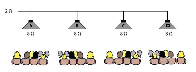
Figure 1 – A zoned, distributed layout using 8 ohm loudspeakers.
Amplifier Types
There are three amplifiers being considered for the project. They are rated as described in Figure 2. The grey text shows the Loading Effect as described in the Common Amplifier Format Reference. It shows the voltage drop caused by the increased load (lower ohms), relative to a reference condition, which in this case is the 8-ohm load.
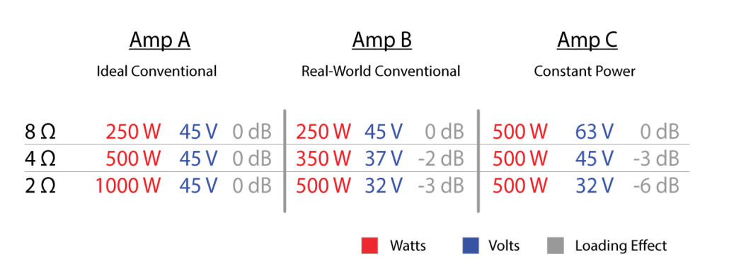
Figure 2 – Three amplifier types compared
“Ideal” Conventional Amplifier
As the techs deploy the system, some program material is fed to the amplifier. The connection is made to Spk A and the amplifier input sensitivity is adjusted to produce the target listening level. Spk B is connected to the parallel jack of Spk A and starts playing. Since the amplifier’s output voltage is unchanged by the added load, the SPL from Spk A is not affected, and Spk B plays at the same level. The process is repeated for Spk C and Spk D, with the SPL from Spk A (and Spk B) unaffected by the presence of C and D.
This amplifier maintains its output voltage and doubles its current (and audio power) for each halving of the load impedance. It is rated to maintain this behavior down to 2 ohms. Note that the 2-ohm load will require very heavy cable, but that’s a different topic.
Real-World Conventional Amplifier
A real-world amplifier, by design, has a limited amount of available current. As the techs deploy the system Spk A is connected and the amplifier adjusted for the target SPL. When Spk B is connected, the SPL from Spk A drops by 2 dB. When Spks C and D are connected, the SPL from Spk A (and B) drops by 3 dB. This behavior is dynamic and program-dependent, with the amplifier essentially behaving as a compressor. Alternately the amplifier just goes into distortion with the increased load. In either case, the amplifier’s behavior is now non-linear.
The designer must still deal with the line loss from the cables.
“Constant Power” Amplifier
A constant power amplifier produces the same audio power into any load impedance. As the techs deploy the system Spk A is connected and the amplifier adjusted for the target SPL. When Spk B is connected, the SPL from Spk A drops by 3 dB. When Spks C and D are connected, the SPL from Spk A drops by 6 dB. This behavior is dynamic and program-dependent, with the amplifier essentially behaving as a compressor. Even though the SPL drops (dynamically) the amplifier can handle the load and doesn’t overheat.
The designer must still deal with the line loss from the cables.
Transformer-Distribution System
The ideal scenario (Amplifier A) can be realized using a transformer-distribution system. Each loudspeaker is connected through a 25o W autoformer. An autoformer is essentially a step-down coil that is smaller and lighter than a transformer. Autoformers are often used in lieu of transformers in high power distribution schemes, such as the one described in this article. Not only would this type of system perform like the ideal scenario, but the line loss due to wire resistance would be reduced since the autoformer makes the 8-ohm load look like 20 ohms to the amplifier. Figure 3 shows a screen capture from the “High-Z Calc” of the CAF Viewer for a single load on the amplifier. Note that the required amplifier size would 1 kW if all four loudspeakers are connected using AWG 13 wire with a home run back to the amplifier for each loudspeaker. Once can simply increase the Qty field to 4 to account for this.
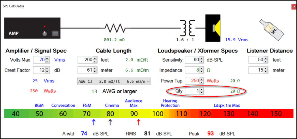 Figure 3 – A transformer distribution approach.
“Self-Powered” Loudspeakers
Another approach would be to use internally-powered loudspeakers. The required “daisy-chaining” is now done at line level ahead of the amplifiers. The impedances are much higher here (measured in kΩ) and line loss is completely mitigated. This approach requires AC power cables in addition to a twisted-pair for the signal. In some cases, the loudspeakers can be AC powered along the route, reduced the required wire gauge for the extension cords.
Subwoofer Array
Since we’ve come this far, there is one more scenario that should be considered. Instead of a parade route, let’s stack all four loudspeakers and make a subwoofer array. The difference is that this sums the acoustic outputs of the loudspeakers, where as before they were isolated. Nothing with change with regard to the amplifier loading or behavior, but we can expect an increase in SPL along with a shaping of the radiation pattern, depending on how the subs are stacked. Due to the long wavelengths at these frequencies the acoustic summing will approach 6 dB per doubling of boxes, or +12 dB overall. Since the ideal case rarely occurs let’s call it +10 dB. This means Amp A and the self-powered subs will yield +12 dB. Amp B will yield +7 dB. Amp C will yield +4 dB. Yes, in all cases you get “more” but this serves to obfuscate the fact that the amplifiers are tanking under the load.
Conclusion
All of these approaches can “work.” It’s the job of the sound system designer to understand the strengths and weaknesses of each, and then select one that makes sense for the application. pb
Leave a Reply
Want to join the discussion?Feel free to contribute!