CAFViewer v1.3 Additions

Some recent additions to the CAFViewer™ app warrant some exposition. I’ll post some more amplifier profiles in early March.

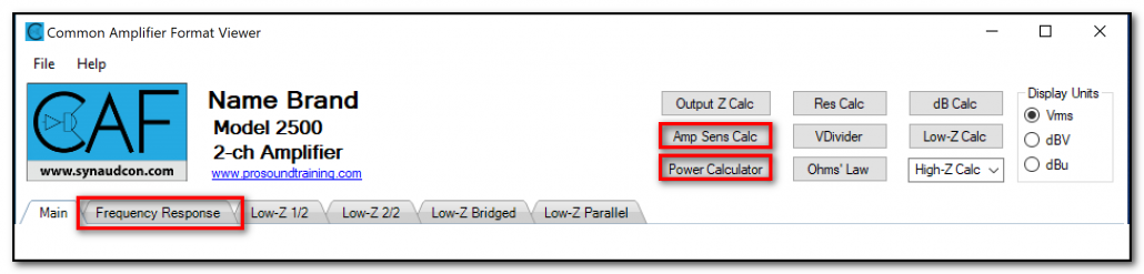
Figure 1 – Some new additions to CAFViewer™ 1.3

Amplifier Sens Calculator
Voltage, current, and resistance are interdependent quantities, conjoined by the power equations. When we drive an amplifier with a voltage waveform, the amplifier produces a higher voltage facsimile of the waveform as per the amplifier’s gain. It must also source sufficient current as demanded by the load resistance. The relationships are relatively simple, but a lot is going on when you consider various load resistances. I designed an interactive calculator for CAFViewer™ that makes the interdependence intuitive, allowing the user to dial up any voltage and see the resultant current and wattage that would be produced by an ideal amplifier – one with sufficient current reserves to maintain the selected voltage as the load resistance is reduced.

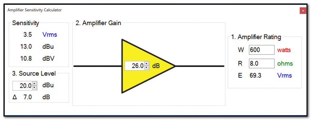
Figure 2 – The new Amplifier Gain calculator shows the relationship between the input and output voltage of the amplifier. It can be used to find the amplifier’s input sensitivity based on the amplifier’s power rating and gain.

Can a real-world amplifier perform this way? No. All audio power amplifiers are current-limited by design and will run out as the load resistance is reduced, resulting in voltage drop, distortion, or both. Many include circuitry that will throttle back the voltage if the current demand exceeds what is available from the amplifier, or what is available from the electrical outlet. For an amplifier to maintain its output voltage into any load resistance, its power must double each time the resistance is halved. When this doesn’t happen, we know that the amplifier has become non-linear and its performance can no longer be described by a simple gain value in dB. An over-loaded amplifier is one that cannot maintain its output voltage due to the load’s demand for current. To complicate matters this behavior is crest factor-dependent.

Power Calculator
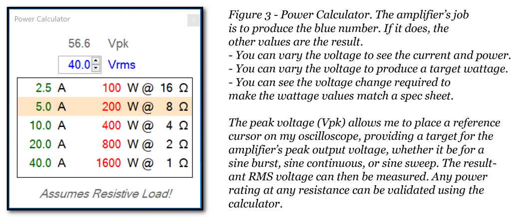
Nearly any low-Z amplifier can hold its voltage into 16-ohms, and that’s the first test I run to find the amplifier’s voltage rails. This voltage can be entered into the new Power Calculator, which shows the current required to drive 16, 8, 4, 2, and 1-ohm loads as well as the resultant wattage.

One ohm? Really? Some automotive amplifiers claim to be able to drive 1-ohm, so I use this calculator to aid in discussions with them. It clearly shows the voltage required to produce a given wattage into the various loads. These are theoretical values, but they provide a reference for progressively loading the amplifier with dummy loads to observe any change to the voltage, stopping at the manufacturers minimum recommended load. On only a few occasions have I loaded an amplifier to 1-ohm to prove that it’s a bad idea.

To summarize, the amplifier’s job is to deliver a voltage to the load. The voltage produces current flow as determined by the load impedance. While power flow is a byproduct of this process, it is not the amplifier’s job to deliver power. If we focus on that we miss the importance of fidelity and linear amplifier behavior.

Scroll your mouse-wheel on the voltage field of the calculator and watch the power change into the various loads. It’s interesting, but not important. Given the impedance curve of the loudspeaker, the power varies dramatically as it is both load and frequency-dependent. Watch the voltage and you’ll see how the amplifier is doing its job.

Free-Form Sweep Tab
The Frequency Response tab of CAFViewer shows the amplifier’s response to a log sweep of one-second duration. Why one second? It’s the minimum period required to assess amplifier power. The CAF process tests the amplifier at its minimum supported impedance, 2x this impedance, and 4x this impedance. So, a “4-ohm” amplifier would be swept at 4, 8, and 16-ohms. A “2-ohm” amplifier would be swept at 2, 4, and 8-ohms. The responses to these sweeps are overlaid and can be very telling regarding the amplifier’s performance as the load resistance is reduced. For a theoretical “ideal” amplifier the sweeps would overlay exactly on top of each other, proving that the amplifier’s output voltage is independent of the load resistance (Figure 4). Figure 5 shows the output voltage of a popular amplifier at progressively lower load resistances. The plot makes it clear at what resistance the amplifier becomes overloaded for the one-second sweep.

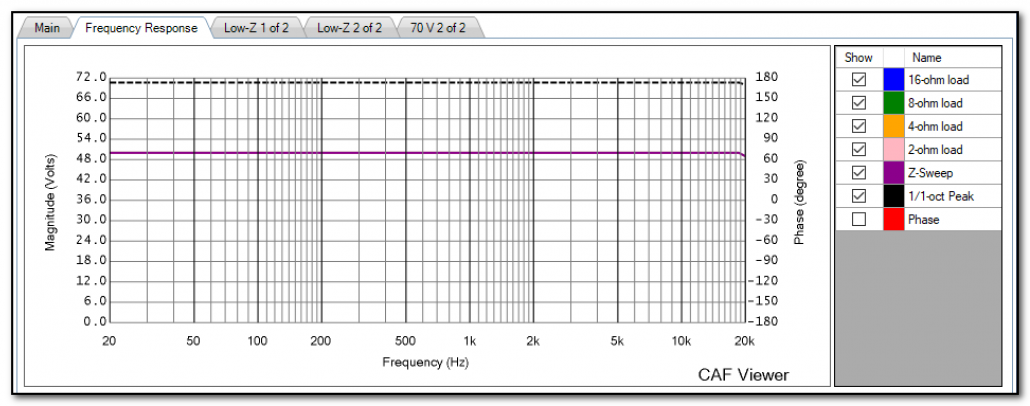
Figure 4 – Overlaid log sweeps of an ideal voltage source. The 16, 8, 4, and 2-ohm plots exactly overlay at 50 Vrms. The peak response (dashed line) is +3 dB relative to the RMS. This is a theoretical amplifier.

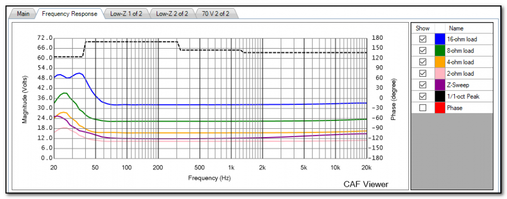
Figure 5 – Overlaid log sweeps of an amplifier with low output current and heavy regulation. Note that the peak voltage (dashed line) is similar to the ideal amplifier.

Conclusion
In conclusion, the CAF provides data for the amplifier’s response using sine burst, sine continuous, and sine sweeps. This paints a complete picture of the amplifier’s performance and clearly shows how the amplifier gets its power rating. As such it provides a way to make meaningful comparisons between makes and models. This body of information is sufficient to assess whether an amplifier is appropriate for a specific application based on the expected load impedance and drive signal type. pb