Common Amplifier Format: MiniDSP PWR-ICE125

by Pat Brown

Overview

The MiniDSP PWR-ICE125 is a 2-channel plate amplifier for active 2-way loudspeakers or subwoofers. Since these articles are tutorial in nature, I’ll use the PWR-ICE125 to present some important fundamentals regarding amplifier ratings and SPL calculations. These same principles can be applied by the reader to the other amplifiers that I have tested in this series.

The Common Amplifier Format (CAF) data file can be downloaded here.

This data is for use in learning and training about audio power amplifiers. It is not intended to augment, supplant, or replace the manufacturer’s published specifications. It has not been approved by the manufacturer.

Operational Modes

The PWR-ICE125 has two operational modes: 2-ch discrete low-Z and 1-ch bridged low-Z (referred to as BTL). The maximum sine wave output voltage is 22 Vrms in discrete mode, and 45 Vrms in bridged mode. The model number (PWR-ICE125) is based on the rated power into 4 ohms.

The IO Matrix (Figure 1) shows the amplifier’s performance at the supported load resistances for burst, continuous, and noise drive signals. The manufacturer only specs 4-ohm performance, but I tested the amplifier at 4, 8, and 16-ohms to assess the output voltage consistency vs. load. The delta-dB column says it all. There is NO variance in output voltage per load or drive signal in the 2-ch discrete mode. This amplifier performs as a true constant-voltage source and will preserve the shape of an audio waveform into its supported loads no matter the crest factor. In my opinion that rating it into 4-ohms in bridged mode is a little ambitious. That’s the equivalent of loading it to 2-ohms in discrete mode, which I would not recommend due to the stress it places on the amplifier. There’s no fan, and it’s likely to be inside a loudspeaker enclosure, which is another name for an oven.

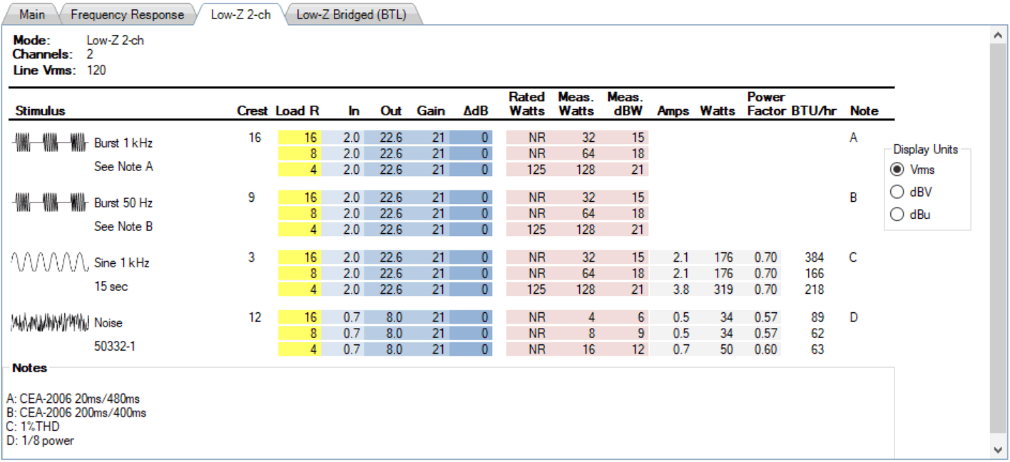
Figure 1 – The IO Matrix for the Low-Z 2-ch operating mode

A Voltage-Optimized Source

An amplifier power rating can be considered to be a scaling factor. It allows the calculation of the SPL increase that can be expected from the amplifier relative to the loudspeaker’s rated sensitivity. A “one number” wattage rating suggests that there are no conditions to this gain – it applies to every signal type into the supported load impedances over the bandwidth of the loudspeaker.

Deviations in the delta-dB column mean that the amplifier’s performance is conditional, as the output level may change for various signal types and loads. For SPL calculations, PWR-ICE125’s performance is not conditional and can be described by a single number. It’s a gain block, and that is a good thing. The voltage gain is 21 dB for any signal type into any rated load.

SPL Calculations from Amplifier Ratings

The amplifier’s gain, along with the loudspeaker’s sensitivity, can be combined to calculate the SPL at 1 meter. From there the inverse-square law can be used to extend that to any distance from the source. I’ll take a detour and provide a few examples.

Let’s consider a loudspeaker with an average sensitivity (L_sens) of 85 dBSPL @ 2.83 Vrms, 1m. We always begin with that, and then factor in the gain from the amplifier.

Method 1:

Method 2:

Method 3:

Method 4:

Methods 1 and 2 are voltage-based. Since the loudspeaker’s sensitivity is referenced to 2.83 Vrms, we need only to factor in the amplifier’s output voltage to get the SPL. Method 1 uses the voltage directly, and Method 2 converts it to dBV, simplifying the calculation to addition and subtraction. In Method 2 the test level for the loudspeaker’s sensitivity (2.83 V, +9 dBV) must be subtracted before adding the amplifier’s level (22 V, +27 dBV). Of course, this could have been done using dBu instead of dBV by adding 2.2 dB to each level.

Methods 3 is based on power. This is the traditional approach but has some caveats. The loudspeaker’s sensitivity was measured at 2.83 Vrms. A resistance of 8-ohms is assumed, which produces a reference power of 1 W by

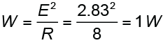
From the CAF IO Matrix the 8-ohm measured power is 61 W. Method 3 calculates the gain from the power ratio and adds it to L_sens to get the SPL at 1 meter.

Method 4 is the same as Method 3, but the wattage rating is first converted to dBW and then simply added to the sensitivity.

Note that all of these values (volts, watts, dBV, dBW) are included in the IO Matrix, along with dBu. Since there is no universal agreement on which to use, the CAFViewer includes them all, letting the user decide. You should get the same SPL using any of them.

IMPORTANT NOTE: For the power methods to work you MUST use the 8-ohm amplifier power. This is because the loudspeaker’s sensitivity is referenced to 2.83 Vrms, which assumes the loudspeaker’s impedance is 8-ohms. A common error is to measure the loudspeaker’s sensitivity at 2.83 Vrms and then consider the amplifier’s 4-ohm (or 2-ohm) power rating when calculating the SPL. While this yields very high SPL, it is wrong. Power-based SPL calculations require that the loudspeaker’s sensitivity is measured using a voltage that produces 1 watt into the loudspeaker’s rated impedance. For a 4-ohm loudspeaker, this would be 2 Vrms, and for a 2-ohm loudspeaker, it would be 1.4 Vrms. Since nearly all low-Z loudspeaker sensitivity ratings are referenced to 2.83 Vrms these days, the power-based methods are obsolete. Due to these caveats, when using watts to calculate SPL the chance for an error is high.

Note that the CAF IO Matrix gives the amplifier power in both watts and dBW, so one simply adds the dBW rating to the loudspeaker’s sensitivity to get the SPL. Simple. Method 4 has the same caveat as Method 3 in that you must use the 8-ohm dBW rating since the loudspeaker’s sensitivity was measured at 2.83 Vrms. MiniDSP does not provide an 8-ohm power rating for this amplifier, so one can either select it from the matrix or assume that it is about ½ the 4-ohm rating.

Don’t Forget the Crest Factor

All of these methods assume a sine wave drive signal (3 dB). It’s already cooked into the ratings. If you are using something else (highly likely) then you must factor that in by adding 3 dB (sine wave crest factor) and then subtracting the CF of your signal. This will reduce the SPL from the sine wave value. If in doubt, 12 dB is a good, general-purpose value for sound reinforcement systems. It assumes a slight limiting/clipping of the audio waveform.

That’s a lot to remember, so all of these variables are readily handled by the CAF’s Low-Z calculator. Just double-click on any voltage in the IO Matrix “Out” column and the calculator will open with that value already entered for the amplifier’s voltage. Enter your loudspeaker’s sensitivity and the signal’s crest factor to complete the SPL calculation (Figure 2).

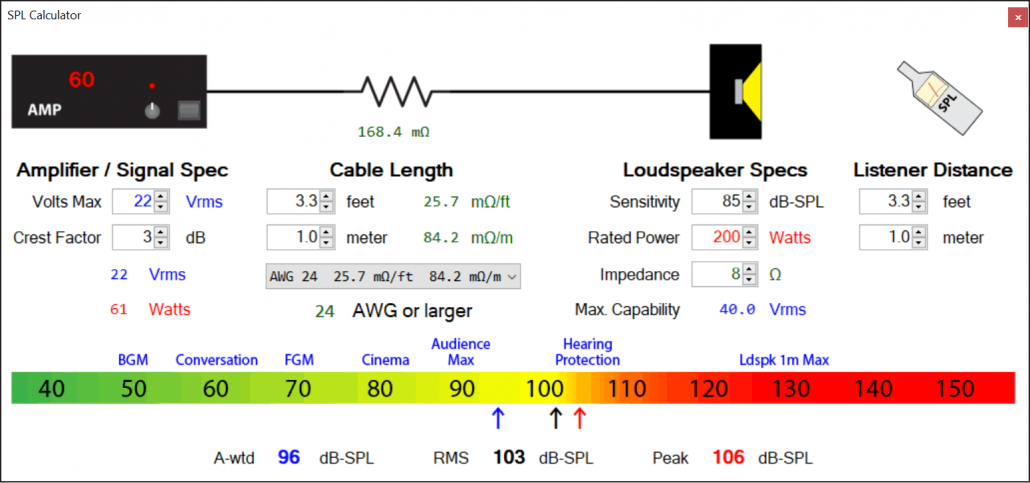
Figure 2 – The CAF Low-Z calculator with the voltage carried over from the IO Matrix.

Push the “Easy” Button

The most accurate (and simplest) way to do SPL calculations is to forget the power and just use the RMS voltage. Wattage ratings create the illusion that you are somehow “getting more” by loading down the amplifier, but in reality, you will get less SPL if the extra load causes the voltage to drop. An audio amplifier whose voltage drops under load is over-loaded.

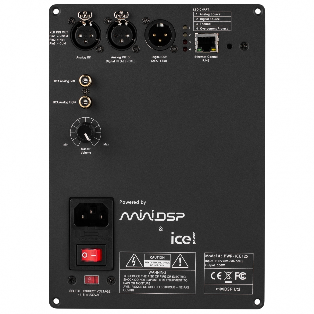
Analog and Digital Inputs

The amplifier has both analog balanced (XLR) & unbalanced inputs (RCA) to provide maximum compatibility. A digital input (AES-EBU) is also provided. A digital output (AES-EBU) allows multiple plate amplifiers to be linked to each other.

The analog input clips at 3.1 Vrms (+12 dBu) at any setting of the analog level control. This means that the amplifier is optimized for a consumer-level signal, which is

-10 dBV + 20 dB = +10 dBV (+12 dBu)

It cannot handle a professional line-level signal, which is

+4 dBu + 20 dB = +24 dBu

even though it provides a professional (XLR) input jack. So, if you try to optimize your system’s gain structure by using the mixer’s full dynamic range and then setting the playback level using the amplifier’s gain control, you’ll get a distorted output with no visual warning from a clip light. So, either back down the mixer or add a pad between it and the amplifier. It’s a common practice to max out the amplifier level control and then set the playback level using the mixer’s level control. While this may prevent over driving the amplifier’s input circuit (due to the reduced mixer level) the overall signal-to-noise ratio (SNR) will suffer. You might get away with that for a live event, but not in a critical listening environment.

On-board Signal Processing

The PWR-ICE125 has a DSP onboard. As the company name suggests, this is one of their strengths. As a registered owner of the amplifier, I can download the PWR-ICE125 control software from the Users section of the MiniDSP website. Both IIR filter-based and FIR filter-based software are available. Both apps provide some standard processing options, along with the ability to import IIR or FIR filter coefficients from 3^rd-party measurement apps and filter-generation utilities such as Filter Hose.

Conclusion

The IO Matrix for the PWR-ICE125 displays its behavior as that of a constant-voltage (CV) source. While this term is sometimes hijacked in recent years to refer to amplifiers designed to drive transformer-distributed loudspeaker systems, the electrical engineering definition has not changed. A CV amplifier’s output voltage is not be affected by the load impedance. Loudspeakers are usually driven by CV amplifiers. In contrast, loop systems for hearing assistance are typically driven by constant current (CC) amplifiers – one whose output current is independent of the load impedance. I’ll use the CAF for some loop amplifiers later in this series.

The PWR-ICE125 is pretty much a textbook amplifier and should be easy to deploy. It has no conditions regarding its performance down to the maximum load of 4-ohms, making it ideal for use in critical listening applications.

This is a nice addition to the CAF article series. pb